Outlier Detection: You have to be ODD to be Number 1

The process of finding data points having great variation from behaviour of the majority of data points in a collection is known as Outlier Detection.

Outliers are actually found in almost any environment in nature. From your classrooms, where a majority of students will score on average good marks, while there will be a few who score exceptionally high. However, let us not confuse between noise and outliers! Noise is just unexpected or temporary variation in data, say for example, in your classroom, students who score exceptionally high but lacks the practical skills to implement its applications. We see outliers and noise in our everyday activities but do not observe them!

Let us take example of sales at our nearest supermarket. The store manager notices that the sales have went down for a certain month so he decides to reduce the prices of the products and suddenly observes a surge in the sales of the month. Now, this sudden rise in sales cannot be termed as an outlier! This is just a temporary variation in the sales and not bound to last for long, infact it may be that customers will stop purchasing if the prices are restored to normal again! This is actually noise!

Let us visualise this in a simple fashion using a scatter plot:

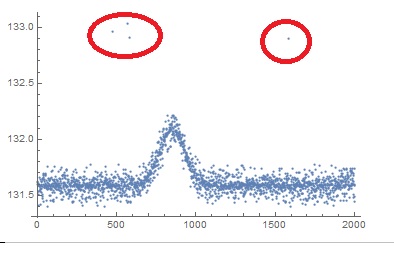
Thus, we can easily see the difference between abrupt noise in the first circular label which indicates abrupt variations and an outlier in the second circular label as shown in the scatter plot. Outliers can be generated from the same process or even different processes. In order to justify, that outliers are made of different processes too, we make assumptions. Say for example, in case of the market transaction, there might be an increase in the sales due to an occassion or festival that led to higher incentive for more people to shop, but it can also be a result of market competition, yet both these processes can lead to generation of outliers in one form or other. Hence, we come to a broader definition of outlier:

The data point(s) which deviate largely from the assumptions made for normal behaviour of data points in a given set can be termed as outliers.

These normal points are clustered together based on the assumptions made on the dataset and any point violating those assumptions is bound to show huge deviation from the cluster and can be isolated as an outlier. Also, the threshold of the deviation can be varied based on the nature of data and other factors. Let us try to learn about the different types of anomalies that exist:

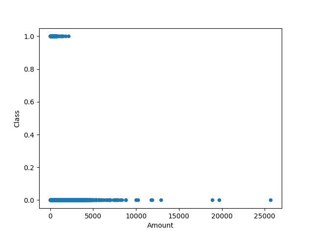
• Global Anomalies: The anomalies which exhibits large scale deviation from the data points and will remain anomalous even with change in contexts or other factors are termed as global anomalies. For example, Credit Card Fraud Detection System where fraudulent transactions are very much different than the legitimate transactions and have a huge deviation in terms of behaviour from normal assumptions. The following is a scatter plot for Amount vs Class (Fraud or Normal) in Credit Card Transaction dataset Link
  
  

• Contextual Anomalies: The anomalies which exhibits changes when subjected to different contexts and are dependent on the nature of data and other factors associated with it are known as contextual anomalies. A great example for this will be a simple question as follows:
  “Is the weather normal today?”
  This question has a very vague answer and has too many behavioural and contextual attributes associated with it. Say for example, the location and the temperature are two classic contextual and behavioural attributes respectively in this case scenario. A 35 degree summer may be normal for a beach in Goa, India but the same will be termed as highly abnormal for say a hill station such as Ooty, India!
  
  

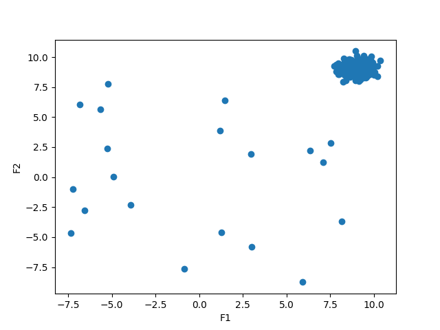
• Collective Anomalies: The anomalies which are found to be a cluster of data points that deviates from the normal behaviour of the majority of data points in the sample are termed to be collective anomalies. For example, if the fraud transactions in a credit card fraud detection system are committed by the same user and using the same set of features to target a specific client then all these transactions will be clustered as an outlier. A simple example using a dummy dataset is plotted as follows:
  
  

Such anomalies are responsible for lowering the classification accuracy of a traditional machine learning model and are more prone to misclassification by any model in general. I have came across many beginners having this doubt that why don’t we just simply drop it? A typical textbook answer to Exploratory Data Analysis, however, not exactly a desirable result!

In some cases, these outliers are very informative and also, it is important for designing a robust machine learning model to be able to classify outliers correctly as well. Consider the case of credit card fraud detection itself, a classic class imbalanced problem where the majority of transactions are legitimate, and only a few transactions are fraud. These fraud transaction exhibits different contextual and behavioural features than legitimate transactions which are hard to define and find. Thus, an outlier analysis becomes significant in such cases. Let us try to understand the concept of handling outliers with credit card fraud detection as a case study.

Suppose you own a bank and need to hire a data scientist for designing a credit card fraud detection system. There are four major possibilities which may occur:

• Actual Fraud, Predicted Fraud: This is the win-win situation where your model was able to find and classify the fraud transaction
• Actual Legitimate, Predited Legitimate: This is to classify normal behaviour of majority of transactions
• Actual Legitimate, Predicted Fraud: This is a problem to the bank as the client may feel irritated, and maybe after a series of clarifications, the customer will be proved innocent. This may lead to wastage of resources but the bank will not incur a much of a loss.
• Actual Fraud, Predicted Legitimate: This is a huge problem as the fraud transaction is left undetected and the client may even file a legal suite against the bank that will lead to a huge loss incurred by the bank. Let us represent this as a confusion matrix:
  

Thus, we can fairly conclude that a model with 99 percent classification accuracy after dropping out the fraud transactions may sound to be the best in textbook definitions, but does not hold true for a real-life scenario. Our model should be able to handle outliers, and be robust enough to predict them correctly even if there are chances of a false negative. So, what we see today in banks is something called Cost Sensitive Learning. A very broad outline defintion borrowed from Jason Brownlee is:

Cost-sensitive learning is a subfield of machine learning that takes the costs of prediction errors (and potentially other costs) into account when training a machine learning model. It is a field of study that is closely related to the field of imbalanced learning that is concerned with classification on datasets with a skewed class distribution.

Let us read between the lines and try to understand what does this say! So, we see something called costs of prediction errors! This refers to the idea polarised compared to traditional machine learning models which try to minimize errors. Instead of trying to classify correctly, we give each instance a value called misclassification cost and the aim of the model is to optimize this misclassification cost. Now, comes the word imbalanced learning. This refers to the idea that a dataset is dominated by a single label more than the other class labels available for classification. This leads to creation of an inherent bias in the model towards that majoritarian label. Say for example, there are millions of legitimate transactions in a bank everyday but only a handful of fraud transactions, thus if we train the model on this data, it might suffer from bias towards legitimate transactions and classify any upcoming transaction as legitimate leaving us more prone to not detecting frauds committed. Thus, we need to solve this problem. But, let us first dive into some code.

Let us start by importing the essential libraries for processing.

# Visualisation Library
from matplotlib import pyplot as plt
import warnings
warnings.filterwarnings("ignore")
import seaborn as sns

# Data Processing Library
import pandas as pd
import numpy as np
from imblearn.over_sampling import SMOTE
from sklearn.preprocessing import StandardScaler
from sklearn.model_selection import train_test_split
# Tensorflow
import tensorflow as tf
from tensorflow.keras.layers import Dense
from tensorflow.keras.layers import Input
from tensorflow.keras.models import Model

We are using the Kaggle Dataset available for Credit Card Fraud Transactions (Link)
We start off by observing the data shape and nature.

df = pd.read_csv("creditcard.csv", encoding="utf-8")
print(df.head())

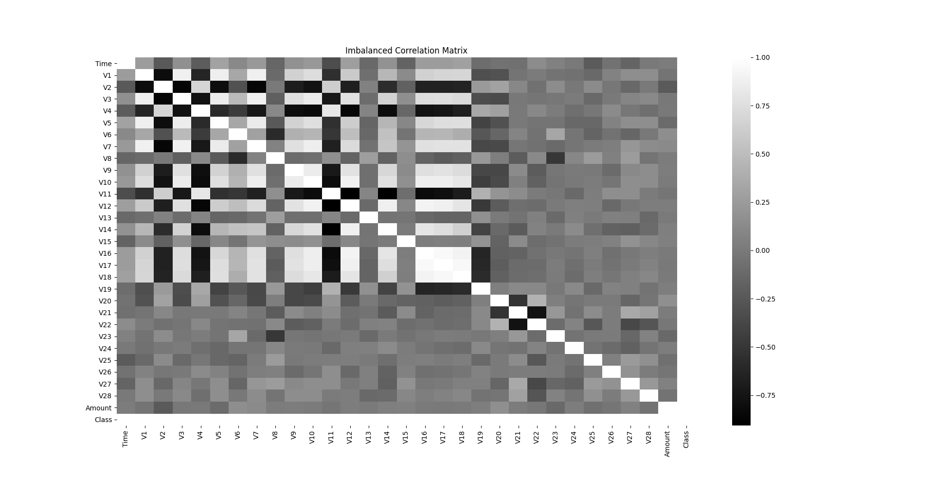
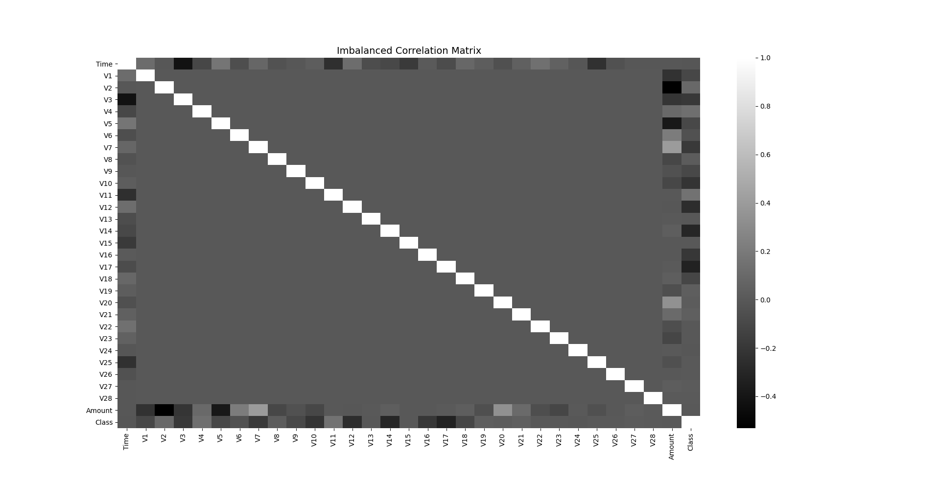
You will observe that we have 32 columns Time, Amount, Class and Features V1 to V28 whose names shall remain confidential to the bank for privacy of customers. Let us try to plot a correlation matrix between all the columns to see a better relationship between them using a heatmap.

fig, ax = plt.subplots(figsize=(20,10))
corr = df.corr()
sns.heatmap(corr, cmap="gray", ax=ax)
ax.set_title("Imbalanced Correlation Matrix", fontsize=14)
plt.show()

We can easily make out poor correlation between features, but let us first see an analysis of the class labels.

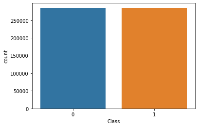
sns.countplot(x='Class', data=df)

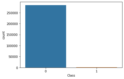
Clearly, the number of legitimate transactions is way too high than the number of fraud transactions and hence it is a class imbalanced problem. Imbalanced datasets needs to be balanced in order to get better relationship between their features and there are a variety of techniques used for that varying from using ensembles, adding weights parameter in algorithms, but here we use a concept called Synthetic Minority Oversampling (SMOTE). SMOTE simply increases the population of minority class by duplicating the instances which may not add any new information to the model. SMOTE works by selecting examples that are close in the feature space, drawing a line between the examples in the feature space and drawing a new sample at a point along that line. It works on the principle of k-nearest neighbours by selecting a certain value for k say k=5, and picks up any instance closely resembling the feature space out of these five instances. This can be used to create many synthetic examples without worrying about influencing the model because it does not provide any additional information to it. The Python Library imblearn provides a prebuilt SMOTE, let us see its use.

sm = SMOTE(sampling_strategy='minority', random_state=7)
resampled_X, resampled_Y = sm.fit_resample(df.drop('Class', axis=1), df['Class'])
oversampled_df = pd.concat([pd.DataFrame(resampled_X), pd.DataFrame(resampled_Y)], axis=1)
oversampled_df.columns = df.columns
oversampled_df['Class'].value_counts()

Now, the data is balanced with no bias towards the majoritarian class and hence, a sample of such data shall be a better representative of the entire population to ensure a robust machine learning model upon training. So, let us plot the correlation matrix and heatmap again to see the difference in relationship among the columns than earlier.

fig, ax = plt.subplots(figsize=(20,10))         
corr = oversampled_df.corr()
sns.heatmap(corr, cmap='gray', annot_kws={'size':30}, ax=ax)
ax.set_title("Imbalanced Correlation Matrix", fontsize=14)
plt.show()

Now, the correlations among the features become much more clearer and easier to analyse. However, we observe that the values of each feature varies highly for comparison. Thus, the natural progressive step will be to standardize these values as to make them suitable for comparison.

sc = StandardScaler()
X = oversampled_df.iloc[:, 1:-1].values
y = oversampled_df.iloc[:, -1].values
y = y.reshape(-1, 1)
print(X.shape, y.shape)
X = sc.fit_transform(X)
print(X[0])

Now, let us split the dataset into train and test sets for running the model.

x_train, x_test, y_train, y_test = train_test_split(X, y, test_size=0.3, random_state=42)

We will try to set up a small neural network to perform binary classification now.

x_features = X.shape[1]
y_features = y.shape[1]

Thus, we get the feature shapes of the given set of data.

adam = tf.keras.optimizers.Adam(learning_rate=0.0005)
i = Input(shape=(x_features,))

x = Dense(64, activation='relu')(i)
x = Dense(64, activation='relu')(x)
o = Dense(y_features, activation='sigmoid')(x)

model = Model(i,o)
model.compile(loss="binary_crossentropy", metrics=['accuracy'], optimizer=adam)
print(model.summary())
callback = tf.keras.callbacks.EarlyStopping(
    monitor='val_loss', min_delta=0, patience=10, verbose=0, mode='auto',
    baseline=None, restore_best_weights=True
)

We make use of an adam optimizer with optimal learning rate not too high nor too low. If we keep the learning rate too high, it may skip useful features in the data and if we keep it too low it will take a very long time to train and possibly even overfit to learn unnecessary complex features. We will get 6145 parameters with the above network which comprises of two dense layers with activation function ‘ReLU’ and a dense output layer as well with binary crossentropy as loss function which needs to be minimized with an adam optimizer. Now, run the model as follow:

r=model.fit(x_train, y_train, epochs=100, batch_size=512, verbose=1, validation_data=(x_test, y_test), callbacks=[callback])

We run it for 100 epochs with an early stopping if we achieve validation accuracy better than 99.5. At the end of it, you will get a model with an accuracy of 99.97 on validation set. Thus, a deployable model and let us try it on test set.

results = model.evaluate(x_test, y_test, batch_size=5, verbose=1)
print("Loss: %.2f" % results[0])
print("Acc: %.2f" % results[1])
y_pred = model.predict(x_test)
y_pred = np.round(y_pred, decimals=0).astype(int)

We will get a test accuracy of 99.98% which is decent and deployable. Let us plot our training history and compare it with the validation set training.

print(r.history.keys())
plt.plot(r.history['loss'])
plt.plot(r.history['val_loss'])
plt.legend(['loss', 'val_loss'])
plt.show()

plt.plot(r.history['accuracy'])
plt.plot(r.history['val_accuracy'])
plt.legend(['accuracy', 'val_accuracy'])
plt.show()

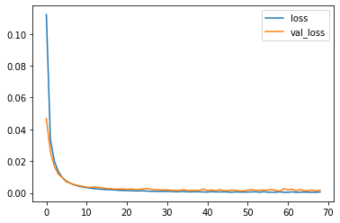
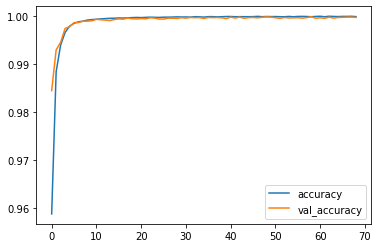
Thus, we observe the network handled training pretty nicely without any overfitting or underfitting! For a complete code, you can refer my colab notebook: Link
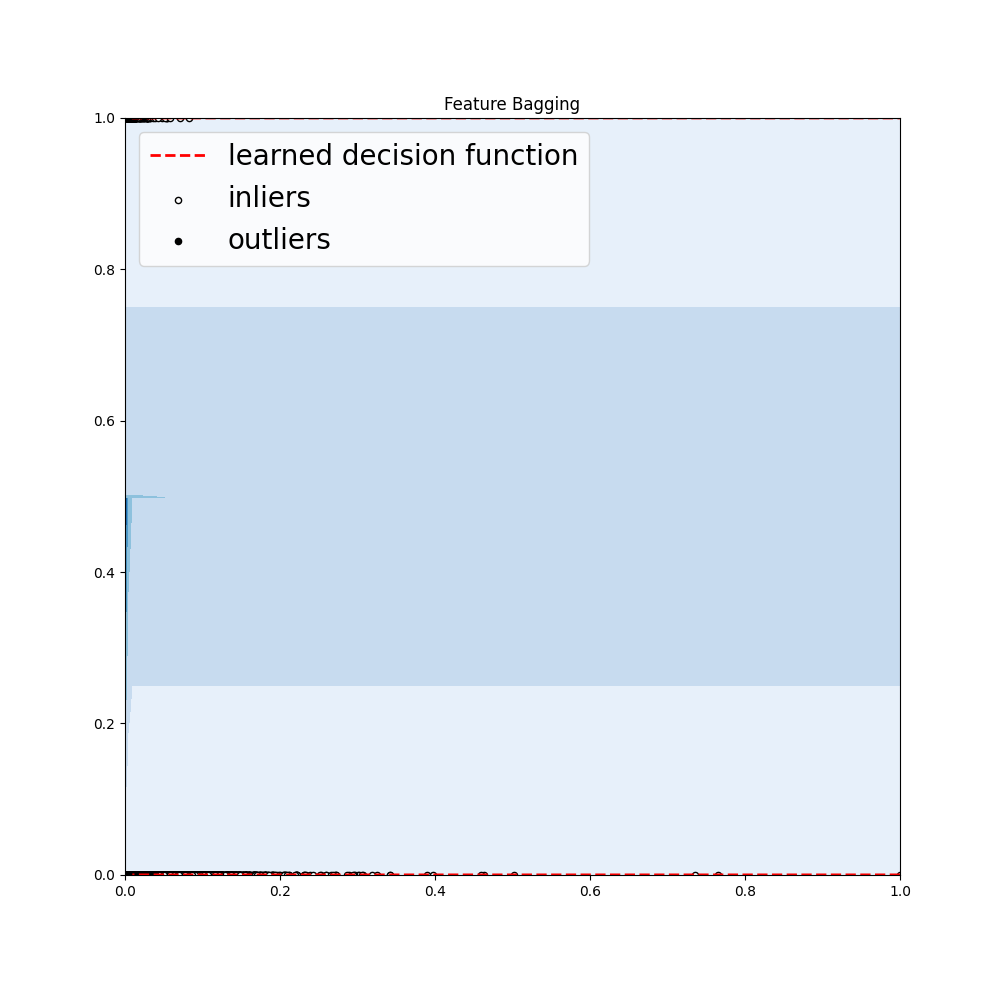
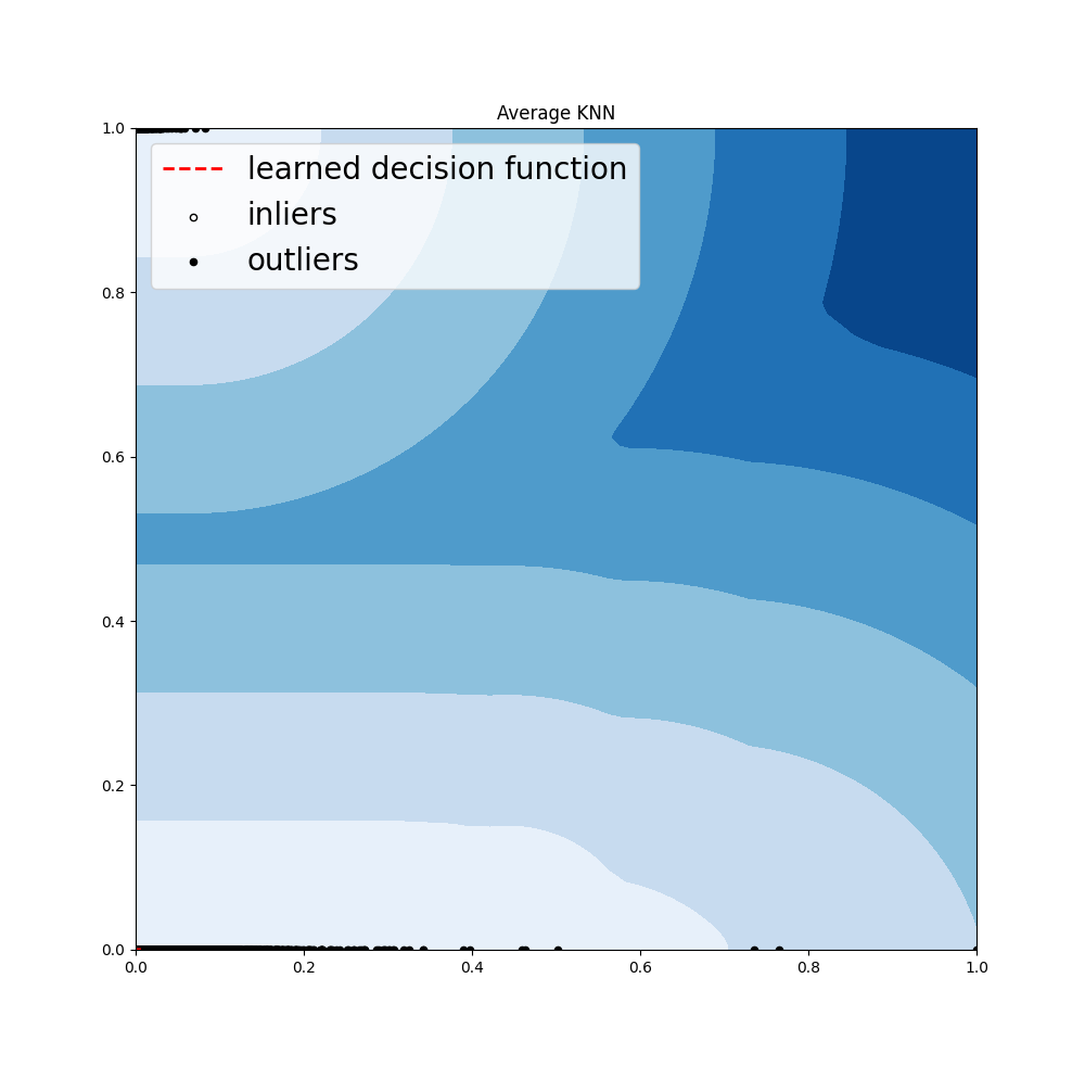
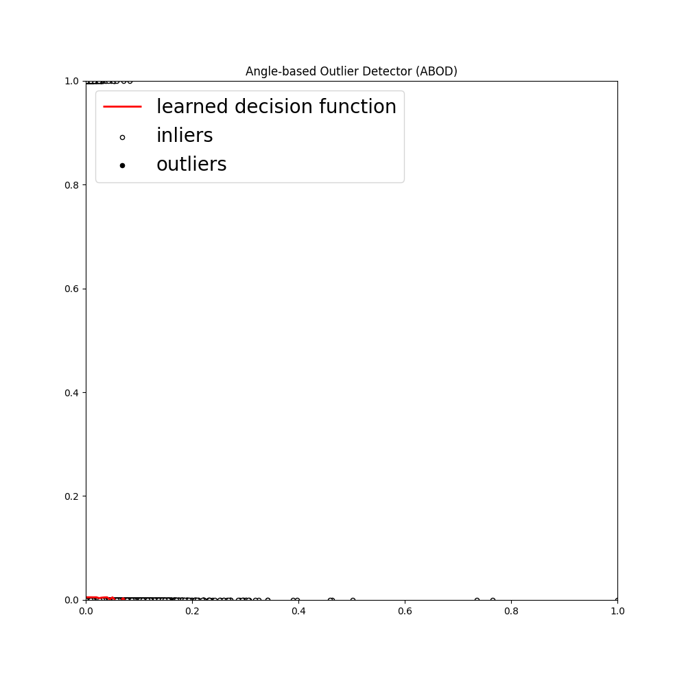
Now, let us get to some theoretical concepts for outlier detection in this problem. CMU created a PyOD library specifically for outlier detection which is makes use the following algorithms:

1. Angle Based Outlier Detection:The notion of ABOD algorithm is to find the outlier based on the variance of the angles between the difference vectors of data objects in the dataset.This way, the effects of the “curse of dimensionality” are alleviated compared to purely distance-based approaches.
   • It considers the relationship of a data point and its neighbours
   • It does not consider the relationship between those neighbours
   • The variance of its weighted cosine scores to all the neighbours could be viewed as outlying score
   • It performs well on multi-dimensional data
   • It is of two major types: Fast ABOD (uses k-nearest neighbours) and Original ABOD (runs on all the training points)
     
     
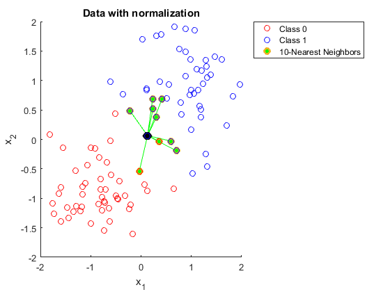
2. k-Nearest Neighbours: Consider the k-nearest neighbours of the given data point and it will be used as the outlying score for that data point. Hence, if any data point has a huge deviation from its neighbours, it can be classified as outlier.
   • It supports three different distance metrics of central tendency: mean, median and mode.
     
     

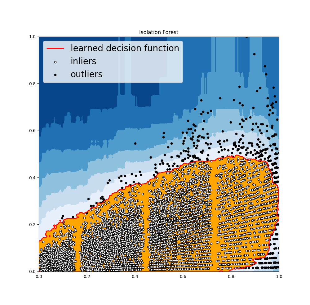
3. Isolation Forest: An algorithm to implement robust decision trees, it takes random features as inputs, splits them based on a random value to ensure no bias and then selects a split between max and min values of the given set of features. In general the first step to anomaly detection is to construct a profile of normal behaviour of points, and then report anything that cannot be considered normal as anomalous. However, the isolation forest algorithm does not work on this principle, it does not define “normal” behavior, and it does not calculate point-based distances. Anomalies are observations that are few and different, which should make them easier to identify. Isolation Forest uses an ensemble of Isolation Trees for the given data points to isolate anomalies.
   
   

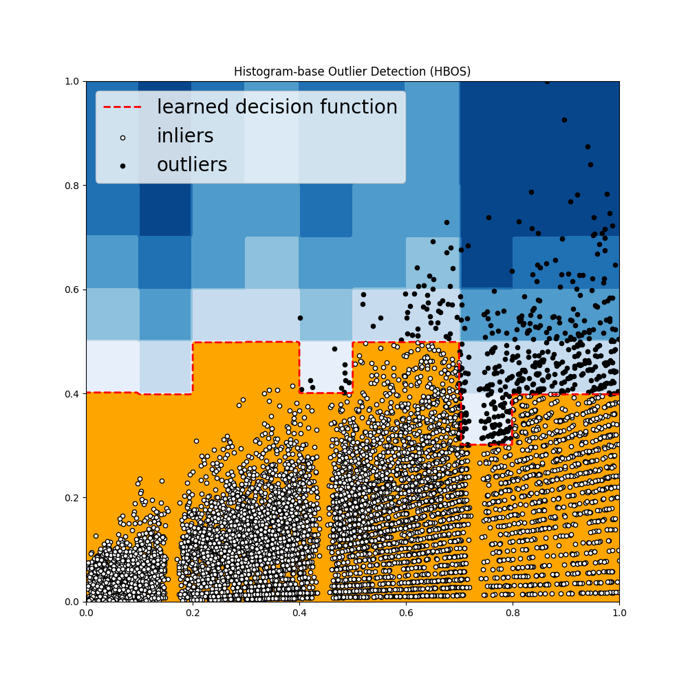
4. Histogram Based Outlier Score Detection (HBOS): It constructs a histogram to efficiently calculate the unusual behaviour present in a feature. It is much faster than multivariate approaches.
   
   

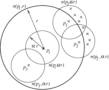
5. Local Correlation Integral (LOCI): Most effective technique in detecting single and group of outliers based on their similarity index and correlation between points that clusters them together. It is a built-in package in PyOD with method generate.data(outliers (uniform distribution), inliers(gaussian distribution)). LOCI computes a counting neighborhood to the nn nearest observations, where the radius is equal to the outermost observation. Within the counting neighborhood each observation has a sampling neighborhood of which the size is determined by the alpha input parameter. LOCI returns an outlier score based on the standard deviation of the sampling neighborhood, called the multi-granularity deviation factor (MDEF). The LOCI function is useful for outlier detection in clustering and other multidimensional domains
   
   

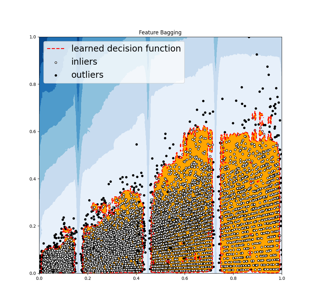
6. Feature Bagging: Feature bagging first constructs n sub-samples by randomly selecting a subset of features. This brings out the diversity of base estimators. Finally, the prediction score is generated by averaging or taking the maximum of all base detectors.
   
   

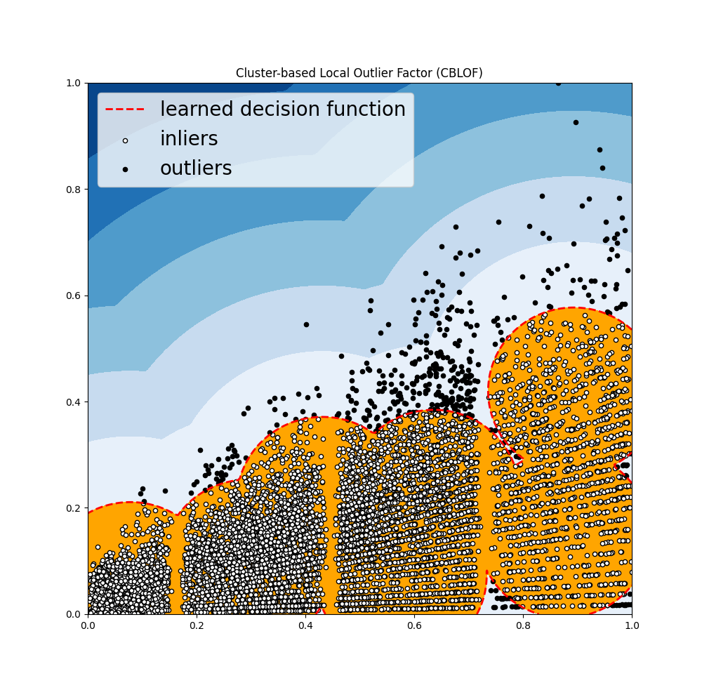
7. Cluster Based Local Outlier Factor: It classifies the data into small clusters and large clusters. The anomaly score is then calculated based on the size of the cluster the point belongs to, as well as the distance to the nearest large cluster.
   
   

Now, let us try our hands on the credit card fraud detection dataset to get outliers using PyOD:

# Import necessary libraries
import pandas as pd
import numpy as np
import matplotlib.pyplot as plt
from pyod.models.abod import ABOD
from pyod.models.cblof import CBLOF
from pyod.models.feature_bagging import FeatureBagging
from pyod.models.hbos import HBOS
from pyod.models.iforest import IForest
from pyod.models.knn import KNN
from pyod.models.lof import LOF
from scipy import stats
import matplotlib
import seaborn as sns

Now, read the dataset and display its features as a scatter plot.

df = pd.read_csv("creditcard.csv")
print(df.columns)
df.plot.scatter('Amount', 'Class')
plt.show()

Once again we will analyse the correlation matrix.

fig, ax = plt.subplots(figsize=(20,10))
corr = df.corr()
sns.heatmap(corr, cmap="gray", annot_kws={'size':30}, ax=ax)
ax.set_title("Imbalanced Correlation Matrix", fontsize=14)
plt.show()

Now, standardize the data!

from sklearn.preprocessing import MinMaxScaler
scaler = MinMaxScaler(feature_range=(0,1))
df[['Amount']] = scaler.fit_transform(df[['Amount']])
X1 = df['Amount'].values.reshape(-1,1)
X2 = df['Class'].values.reshape(-1,1)

X = np.concatenate((X1, X2), axis=1)

random_state = np.random.RandomState(42)
outliers_fraction = 0.05

Now, we will declare the classifiers of package PyOD.

classifiers = {
        'Angle-based Outlier Detector (ABOD)': ABOD(contamination=outliers_fraction),
        'Cluster-based Local Outlier Factor (CBLOF)':CBLOF(contamination=outliers_fraction,check_estimator=False, random_state=random_state),
        'Feature Bagging':FeatureBagging(LOF(n_neighbors=35),contamination=outliers_fraction,check_estimator=False,random_state=random_state),
        'Histogram-base Outlier Detection (HBOS)': HBOS(contamination=outliers_fraction),
        'Isolation Forest': IForest(contamination=outliers_fraction,random_state=random_state),
        'K Nearest Neighbors (KNN)': KNN(contamination=outliers_fraction),
        'Average KNN': KNN(method='mean',contamination=outliers_fraction)
}

Make a mesh grid for same.

xx , yy = np.meshgrid(np.linspace(0,1 , 200), np.linspace(0, 1, 200))

And the rest is simply to make plots and call the classifiers one by one!

for i, (clf_name, clf) in enumerate(classifiers.items()):
    clf.fit(X)
    scores_pred = clf.decision_function(X) * -1
        
    # prediction of a datapoint category outlier or inlier
    y_pred = clf.predict(X)
    n_inliers = len(y_pred) - np.count_nonzero(y_pred)
    n_outliers = np.count_nonzero(y_pred == 1)
    plt.figure(figsize=(10, 10))
    dfx = df
    dfx['outlier'] = y_pred.tolist()
    
    # IX1 - inlier feature 1,  IX2 - inlier feature 2
    IX1 =  np.array(dfx['Amount'][dfx['outlier'] == 0]).reshape(-1,1)
    IX2 =  np.array(dfx['Class'][dfx['outlier'] == 0]).reshape(-1,1)
    
    # OX1 - outlier feature 1, OX2 - outlier feature 2
    OX1 =  dfx['Amount'][dfx['outlier'] == 1].values.reshape(-1,1)
    OX2 =  dfx['Class'][dfx['outlier'] == 1].values.reshape(-1,1)
         
    print('OUTLIERS : ',n_outliers,'INLIERS : ',n_inliers, clf_name)
        
    # threshold value to consider a datapoint inlier or outlier
    threshold = stats.scoreatpercentile(scores_pred,100 * outliers_fraction)
        
    # decision function calculates the raw anomaly score for every point
    Z = clf.decision_function(np.c_[xx.ravel(), yy.ravel()]) * -1
    Z = Z.reshape(xx.shape)
          
    # plotting
    plt.contourf(xx, yy, Z, levels=np.linspace(Z.min(), threshold, 7),cmap=plt.cm.Blues_r)
        

    a = plt.contour(xx, yy, Z, levels=[threshold],linewidths=2, colors='red')
        

    plt.contourf(xx, yy, Z, levels=[threshold, Z.max()],colors='orange')
        
    b = plt.scatter(IX1,IX2, c='white',s=20, edgecolor='k')
    
    c = plt.scatter(OX1,OX2, c='black',s=20, edgecolor='k')
       
    plt.axis('tight')  
    

    plt.legend(
        [a.collections[0], b,c],
        ['learned decision function', 'inliers','outliers'],
        prop=matplotlib.font_manager.FontProperties(size=20),
        loc=2)
      
    plt.xlim((0, 1))
    plt.ylim((0, 1))
    plt.title(clf_name)
    plt.show()

And we will get some of the following outputs:



For all the outputs, try out the code yourself! Hence, we learnt about outliers, why and how they exist, how can we detect them and how to deal with them in machine learning models. Try it out on different datasets and happy learning!