Introduction

What is Linear? A linear equation is something which has two variables, one dependent and one independent variable along with a constant term. Let’s say you go out to buy something. The price of the item which you want to buy is affected by the supply of items available. But the cost of travelling to the supermarket is included in every case and is constant from your home provided the constraints like the distance between two places and remains constant and there are less fluctuations in the fuel prices. Here, the cost of items is dependent variable, the supply of items is independent variable which affects the dependent variable and the cost of travelling is the constant. The equation can thus be represented in the form of y = mx + b, which is the linear equation of a straight line.

Linear Regression is usually the first machine learning algorithm which is a data scientist learns. It is a powerful technique to analyse data and make predictions using that analysis. The aim is to find relationship between one or more features(independent variables) and a target or dependent variable. This process is called Simple or Univariate Linear Regression for one feature and Multiple Linear Regression for multiple features. We will discuss simple Linear Regression in this blog.

The Hypothesis/Theory/Concept/Mathematics/Part which is NOT THE CODE BUT IMPORTANT

The relationship between two variables can be represented in the form of a straight line y=mx + b. Here, m is the slope of the line and b is the y-intercept and gives the value of y(dependent variable) when x(independent variable)=0. The slope m is the rate of change of y with respect to x and can be found out by differentiating y with respect to x i.e. dy/dx (calculus,yes.) 🤓

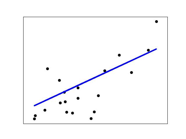
We cannot change the data features, so the values of x and y cannot be changed. The values of slope m and intercept b is in our control. But based on this, there can be any number of values of y whih can be predicted and any number of lines which can be plotted. The regression algorithm gives the line which fits the data points in the best possible way. A multiple regression model can be represented in the form of an equation as follows :

            y = m0x0 + m1x1 + m2x2 + m3x3 + ...... + mnxn + b. 
            b is the bias term,
            m0,m1,m2,....mn are the parameters and
            x0,x1,x2,.....xn are the features values. 

In case of three variables, the equation is a plane. Here, the equation results in the form of a hyperplane.

Let us Begin

For creation of a properly running, efficient regression model, there are three steps:

1. Preparing the data and coding
2. Training the model
3. Evaluating and visualising the model

We will make use of Scikit-learn and Matplotlib. Scikit-learn is a free and open source Python library designed to work with SciPy and NumPy and features various regression, classification and clustering algorithms. Matplotlib is a plotting library in Python and its extensions like SciPy and NumPy and provides API for embedding plots into apps. You can generate histograms, bar charts, plots etc. with this. The installation can be found in the following documentations:

Sckikit-learn : https://scikit-learn.org/stable/install.html  
Matplotlib : https://matplotlib.org/users/installing.html

model.py

import matplotlib.pyplot as plt
from sklearn import linear_model # contains linear regression module

X = [[1.47], [1.50], [1.52], [1.55], [1.57], [1.60], [1.63], [1.65], [1.68], [1.70], [1.73], [1.75], [1.78], [1.80], [1.83], [1.82]]

Y = [52.21, 53.12, 54.48, 55.84, 57.20, 58.57, 59.93, 61.29, 63.11, 64.47, 66.28, 68.10, 69.92, 72.19, 74.46, 58]

reg = linear_model.LinearRegression() # our regression module
reg.fit(X, Y) # make it learn the data

a = reg.coef_[0] # the a value is stored as coefficient
b = reg.intercept_ # the b value is stored as intercept

ablineValues = [] # this list stores the predicted value for all points
for i in X:
 ablineValues.append(a * i[0] + b)

plt.scatter(X, Y) # plot the points
plt.plot(X, ablineValues) # plot the line
plt.show() # show the plot

• We start with importing the libraries and the required functions. The matplotlib.pyplot is a function in the matplotlib library which provides a MATLAB like plotting frame. The alias plt is used. From the scikit-learn library, linear_model is imported, which contains the LinearRegression() module which we will see later.

• After this the data is prepared and stored in the form of lists in Python. The linear_regression model makes use of LinearRegression() module and stores the returned value in a variable named “reg”. The LinearRegression() module has four parameters namely:

  1. fit_intercept(calculates intercept when True,default value:True)
  2. normalize(regressors X normalized before regression if True, default value: False)
  3. copy_X(X will be copied if True, else overwritten, default value: True)
  4. n_jobs(number of jobs that can be used for computing large problems)

  All these are optional parameters. Along with this there are two attributes: coef_ and intercept_ which give the coefficients and intercept terms in the linear regression model.

• The fit() function is called with “reg” and is used to fit the data and is used for training the model. The parameters for this fit method are self, X(array_like or sparse matrix, shape(n_samples, n_features)) which is the Training data, y(array_like, shape(n_samples,n_targets)) which shows target values, sample_weight(numpy array) which shows weight values for each sample. Self returns an instance of self.

• The coefficient and intercept values found are stored in variables a and b respectively. The predicted values for all points are stored in a list named “ablinevalues”(the values returned from linear equation). The values of dependent variables for each point can be found by running a for loop through all X values and appending the result to the list.

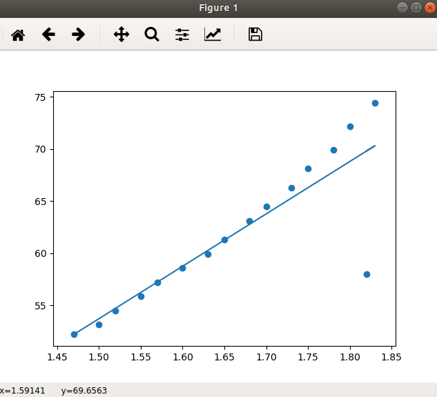
• Next we use scatter() method of matplotlib to plot the points. We use anothe visualise.py program to visualise the available data. The line is then plotted using the input variable X values along with the list ablinevalues in which predicted values are stored. We use plot() method to do this. Then, the show() method is applied to show the plot of points and the line which best fits them.

visualise.py

 import matplotlib.pyplot as plt

X = [1.47, 1.50, 1.52, 1.55, 1.57, 1.60, 1.63, 1.65, 1.68, 1.70, 1.73, 1.75, 1.78, 1.80, 1.83, 1.82]

Y = [52.21, 53.12, 54.48, 55.84, 57.20, 58.57, 59.93, 61.29, 63.11, 64.47, 66.28, 68.10, 69.92, 72.19, 74.46, 58]

plt.scatter(X, Y)
plt.show()

• The output looks as follows:

• In this way, we implement linear regression on a set of data points and train our model. next comes, the evaluation of our model. This is the final step. This is important to judge how a particular algorithm performs on a given dataset. For regression algorithms, three metrics are used :

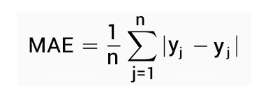
Mean Absolute Error(MAE)- Mean of the absolute value of errors. Calculated as:

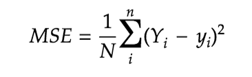
Mean Squared Error(MSE)- Mean of squared errors. Calculated as:

Root Mean Square Error(RMSE)- Square root of mean of squared errors. Calculated as:

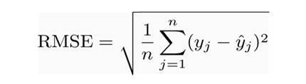
The scikit learn library provides inbuilt functions for calculating these values so you don’t have to calculate them manually. The line for which the error between the predicted values and the absolute value is the minimum is called the best fit line or regression line. The errors are called residuals and can be visualised by using vertical lines which denote the distance between the line and the observed values.

The errors may predict the accuracy of the model. Any kind of inaccuracy in a model is because of the following three reasons:

1. Less data available- Huge dataset leads to better predictions by the model.
2. Assumptions- The assumptions that the data may or may not follow the linear regression model decides a lot when it comes to accuracy.
3. Relationship between features and target values- The relationship between the predicted values and features must be in enough correlation with each other to give proper results.

Conclusion

You have learnt and implemented a model for your first algorithm in ML with the help of this blog. The visualisation can be improved and you can move forward with the mathematical concepts of Gradient descent algorithm for optimization and evaluation of the model. The entire code is available here.