Open Computer Vision is a simple library aimed at computer vision programming in real time.

Started by Intel in 1999, OpenCV has evolved since then and today has transformed to be one of the most sought preprocessing frameworks for Deep Learning with the onset of neural networks in the recent trends. OpenCV is a wonderful framework for image processing and image augmentation and is primarily useful for training neural networks.

Images

Reading and Displaying of Images

OpenCV provides various methods for this purpose:

• cv2.imread(): To read an image

• cv2.waitKey(): For waiting indefinitely, the argument passed is 0 otherwise can be any number as a keyboard event say for example, 5000 for 5 seconds.

• cv2.imshow(): To display an image

• cv2.destroyAllWindows(): Terminates all the windows created for purpose of resource management.

• cv2.imwrite(): This method is used to save an image in the memory as a file format.

Videos

For recording live video, we create a VideoCapture() object with 0 passed as an argument to it. If we wish capture a specific video file, we can also pass the index or name of the video file as the argument to the VideoCapture() function which can serves as its object.

The following methods are used for Video Processing:

• cv2.VideoCapture(): object to capture the video which returns a boolean value of True if the video is read correctly and False if the video is not read properly.

• cap.read(): returns a bool value whether the frame can be read or not and second returned value is indicating if the frame is actually the frame or not.

• cv2.cvtColor(frame, cv2.COLOR_PROPERTY): It is the OpenCV operation used to apply any color property to the video say for example of converting the frame from BGR to grayscale frame we make use of cv2.COLOR_BGR2GRAY.

Drawing Tools

OpenCV provides tools to construct shapes of different sizes, orientation, position and even write text on them.

Some of the methods used for this are:

• cv2.line: Draws on the image read a line from (x1, y1) to (x2, y2) with the given Color and mentioned thickness.

    eg. `cv2.line(image_name, (0,0), (512,512), (255, 0, 0), 5)` draws a line on the specified image from (0,0) to (512,512) of color Blue and of the thickness 5 pixels.
  

• cv2.rectangle: Draw a rectangle on image read with (x1, y1) as Top-Left coordinate and (x2, y2) as the Bottom-Right coordinate with the specified color and edge thickness.

    eg. `cv2.rectangle(image_name, (350,0), (512,128), (255, 0, 0), 5)` draws a rectangle of the specified image name from the top left corner (350,0) to bottom right corner (512,128) with blue color of the thickness 5 pixels.
  

• cv2.circle(image_name, centre coordinate, radius, color, filling): Draws a circle of from centre and fills it.

    eg. `cv2.circle(image_name, (50,50), 65, (255, 0, 0), -1)` is the circle drawn from the centre (50,50) with radius of 65 and of blue color with the fully filled.
  

• cv2.ellipse():Draws an ellipse from top left to bottom right with the rotation specified angle and the start and end angles too.

    eg. `cv2.ellipse(img,(256,256),(100,50),0,0,180,255,-1)` draws an ellipse with (256, 256) as center, (100, 50) as (major,minor) axis, rotated (0) degrees, with (0, 180) as start angle and end angle with Blue color (255) and filled completely.
  

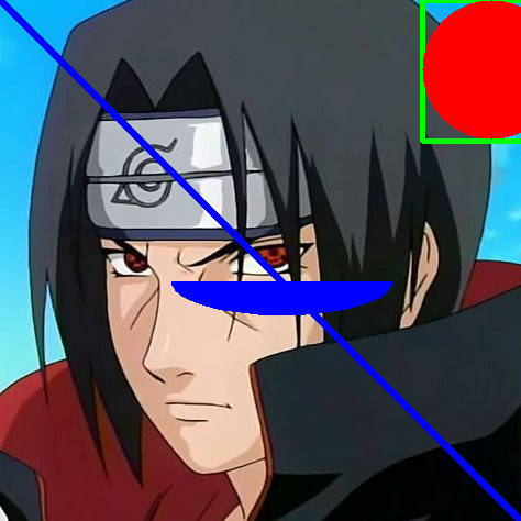
Image Processing Operations

Every image can be represented as an array of pixels in form of a matrix using Numpy Library in Python. After reading of the image, we make use of the rows and columns values to access a certain pixel value. For a RGB image, the order of pixels is BGR and returns Blue, Green and Red Pixels. If the image is grayscaled then the corresponding intensity is returned.

Image Properties

1. Rows
2. Columns
3. Channels
4. Type of Image or Format
5. Number of pixels

If the shape of the image is accessed by img.shape then it returns the number of rows, columns and number of channels in the image.

If the image is grayscale then the tuple returned is containing only number of rows and columns and thus, this acts as a check whether the loaded image is gray scaled or colored image.

The total number of pixels is accessed by img.size

Image Datatype is obtained by img.dtype which returns the format.

Region of Interest or ROI

The feature extraction is an important property of machine learning and image processing and even is important in data mining.

The region of interest is an area in which the useful features are found more conveniently and is used as an approach to enhance the accuracy of the classifier. For example, if we are trying to do face recognition and detection then we make use of an approach where the features on face that can be eyes, nose and mouth are more prominently detected compared to the gradients, scenes and background around it. This helps in improving the accuracy as the search is constrained to a smaller area and it can be obtained simply by using Numpy Indexing.

Arithmetic Operations on Images

Image Addition

cv2.add() or simple numpy addition operation where the result image = image1 + image2

Both the images are of same depth and type while the second image is just a scalar value.

However, the major distinguish feature between these two methods of addition is that the OpenCV Addition is saturated operation while the Numpy addition is more of a modulo operation. Say for example, in OpenCV we have $x=250$, $y=10$ then cv2.add(x, y) = 255 while the numpy result is $x+y = 260$.

Image Blending

In order to blend or mix two images we make use of cv2.addWeighted and can assign weights to each image as well.

Bitwise Operations

• AND

• OR

• NOT

• XOR

Used for creating ROI in different images

Coloring and Object Tracking

The images in open computer vision generally have the following properties that are:

1. Color
2. Hue
3. Saturation
4. Value or Brightness

For any color conversion, we use the function cv2.cvtColor(input_image, flag) which determines the type of the color conversion.

Some of the flags are:

1. COLOR_RGB2RGBA
2. COLOR_RGB2BGR
3. COLOR_RGB2LUV
4. COLOR_RGB2GRAY
5. COLOR_RGB2HSV

For any color detection, we have the following steps to perform:

1. Read all frames in the video
2. Convert from BGR to HSV color space
3. Threshold the HSV image for a range of blue color
4. Extract the blue object alone and do whatever on that image we wish to have

Transformations of Images

Scaling

It is simply resizing of the images which makes use of cv2.resize() for the purpose. This size of image can be specified manually or we can also specify the scaling factor. Preferable interpolation methods are cv2.INTER_AREA for shrinking and cv2.INTER_CUBIC(slow) and cv2.INTER_LINEAR for zooming. By default, we make use of cv2.INTER_LINEAR for any such use.

Translation

The process of shifting the coordinates of an object from one place to other is called translation. It is created in form of a translation matrix.

Perspective Transformation

For perspective transformation, we make use of 3x3 transformation matrix and in which the straight lines will remain straight even after the transformation. To find this transformation we just make use of the points of ROI selected in the image and its corresponding points in the output image. It is performed by the function cv2.getPerspectiveTransform() and followed by applying cv2.warpPerspective() to the tranformation matrix obtained.

Rotation

The process of rotation involves shifting the object with respect to an angle on the axis of rotation. This is done by translating the object to its current axis followed by rotating it about that axis and finally translating it back with respect to the new axis.

Affine Transformation

In this case, all parallel lines in the original image will remain parallel lines in the output images too. To calculate the transformation matrix, we take 3 points on the input image and get their corresponding points on the output image too. Then, we make use of cv2.getAffineTransform() followed by cv2.warpAffine().

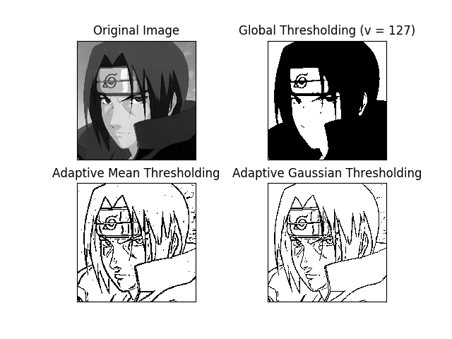
Image Thresholding

Simple Thresholding

If in any image, the pixel value is greater than the threshold value, it is assigned one value otherwise it is assigned another value. OpenCV provides a method `cv2.threshold(image, threshold_value, max_value, type_of_thresholding)`. The fourth argument has many possibilities including:

1. cv2.THRESH_BINARY

2. cv2.THRESH_BINARY_INV

3. cv2.THRESH_TRUNC

4. cv2.THRESH_TOZERO

5. cv2.THRESH_TOZERO_INV

Adaptive Thresholding

In all the images, the illumination of the image may vary and thus we cannot make the global value as the threshold value rather need a method of thresholding which can take into account a specific region of interest. We take the case of adaptive thresholding in which we calculate the threshold values for different regions with different illuminations which leads to a better output. It can have three possible variations:

1.  cv2.ADAPTIVE_THRESH_MEAN_C(): Calculates the mean of the neighbourhood area.

2. cv2.ADAPTIVE_THRESH_GAUSSIAN_C(); The threshold value is the sum of neighbourhood values where weights are a Gaussian Window.

Block-size: It emphasises on the size of the neighbourhood area.	

Otsu Binarization

The only way of verifying whether a threshold value is good or not has been hit and trial so far clearly not so efficient. Consider a simple bimodal image whose histograms has atleast two peaks. So, it automatically calculates the binary threshold value from the histogram peak value. For this, we pass an extra argument of cv2.THRESH_OTSU as flag in the cv2.threshold() method.

Edge Detection

Canny Edge Detector

1. Noise Reduction with a 5x5 Gaussian filter
2. Calculate intensity gradient of the image
3. Perform non-maximum suppression
4. Hysteresis Thresholding

The above steps can be relevantly explained as follows:

The edges of an image are vulnerable to the noises so that the first step would be to remove the noises from the images with a 5x5 gaussian filters and then further subject the smoothening of images with a sobel kernel in both horizontal and vertical direction to get two derivatives say G(x) and G(y) from which we can find edge gradient and direction for each pixel as follows:

$Edge Gradient (G) = \sqrt{G(x)^2 + G(y)^2}$

Hence, the gradient direction will be always perpendicular to the edges. It is rounded to one of the four angles representing the vertical, horizontal and two diagonal directions.

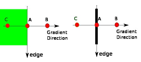
After getting gradient magnitude and direction, we obtain a full scan image to remove all other unwanted edges. For this, at every pixel, pixel is checked for local maximum in its neighbourhood in the direction of gradient. This stage is used to obtain binary images with thin edges.

Hysteresis Thresholding is the stage which decides which are all edges are actually the edges and which are not. It takes two threshold values minVal and maxVal. Any edges with the intensity gradient more than maxVal are sure to be edges and those below minVal are sure to be non-edges based on their connectivity.

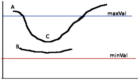
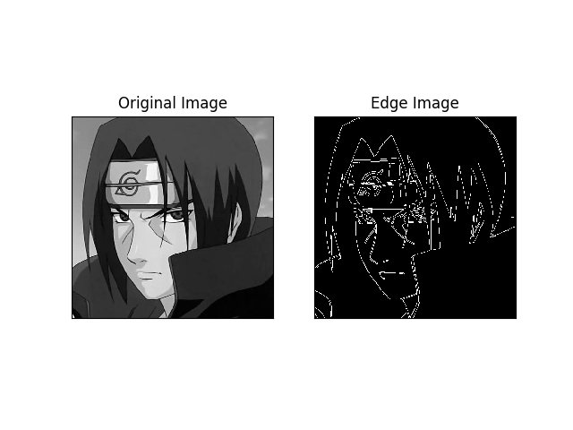
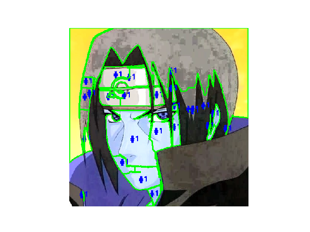
Image Segmentation with Watershed Algorithm

Any grayscale image can be viewed as a topographic surface where high intensity denotes peaks and hills while low intensity denotes valleys. You start filling every isolated valleys (local minima) with different colored water (labels). As the water rises, depending on the peaks (gradients) nearby, water from different valleys, obviously with different colors will start to merge. To avoid that, you build barriers in the locations where water merges. You continue the work of filling water and building barriers until all the peaks are under water. Then the barriers you created gives you the segmentation result. This is the “philosophy” behind the watershed. But this approach gives you oversegmented result due to noise or any other irregularities in the image. So OpenCV implemented a marker-based watershed algorithm where you specify which are all valley points are to be merged and which are not. It is an interactive image segmentation.

Consider any image to be a topographic surface.

If we flood this surface from its minima and prevent the merging of waters coming from different sources, we partition the image into two different sets: The catchement basins and watershed lines. If we apply this transformation, the catchment basin should theoretically correspond to the homogeneous grey level regions of the image and also this may result in over segmentation due to noise or irregularities in the gradient image.

This can be further improved with the use of markers and we can use these markers to control the flooding of the topographic surface, doing so we prevent the over segmentation.

Background Subtraction

It is a major preprocessing step for any vision based application. This helps in making arrangements for extracting the objects from the gradients and scenes behind the target objects.